14 Geomarketing
Prerequisites
- This chapter requires the following packages (tmaptools must also be installed):
library(sf)
library(dplyr)
library(purrr)
library(terra)
library(osmdata)
library(spDataLarge)
library(z22)
As a convenience to the reader and to ensure easy reproducibility, we have made available the downloaded data in the spDataLarge package.
14.1 Introduction
This chapter demonstrates how the skills learned in Parts I and II can be applied to a particular domain: geomarketing (sometimes also referred to as location analysis or location intelligence). This is a broad field of research and commercial application. A typical example of geomarketing is where to locate a new shop. The aim here is to attract most visitors and, ultimately, make the most profit. There are also many non-commercial applications that can use the technique for public benefit, for example, where to locate new health services (Tomintz et al. 2008).
People are fundamental to location analysis, in particular where they are likely to spend their time and other resources. Interestingly, ecological concepts and models are quite similar to those used for store location analysis. Animals and plants can best meet their needs in certain ‘optimal’ locations, based on variables that change over space (Muenchow et al. (2018); see also Chapter 15). This is one of the great strengths of geocomputation and GIScience in general: concepts and methods are transferable to other fields. Polar bears, for example, prefer northern latitudes where temperatures are lower and food (seals and sea lions) is plentiful. Similarly, humans tend to congregate in certain places, creating economic niches (and high land prices) analogous to the ecological niche of the Arctic. The main task of location analysis is to find out, based on available data, where such ‘optimal locations’ are for specific services. Typical research questions include:
- Where do target groups live and which areas do they frequent?
- Where are competing stores or services located?
- How many people can easily reach specific stores?
- Do existing services over- or under-utilize the market potential?
- What is the market share of a company in a specific area?
This chapter demonstrates how geocomputation can answer such questions based on a hypothetical case study and real data.
14.2 Case study: bike shops in Germany
Imagine you are starting a chain of bike shops in Germany. The stores should be placed in urban areas with as many potential customers as possible. Additionally, a hypothetical survey (invented for this chapter, not for commercial use!) suggests that single young males (aged 20 to 40) are most likely to buy your products: this is the target audience. You are in the lucky position to have sufficient capital to open a number of shops. But where should they be placed? Consulting companies (employing geomarketing analysts) would happily charge high rates to answer such questions. Luckily, we can do so ourselves with the help of open data and open source software. The following sections will demonstrate how the techniques learned during the first chapters of the book can be applied to undertake common steps in service location analysis:
- Tidy the input data from the German census (Section 14.3)
- Convert the tabulated census data into raster objects (Section 14.4)
- Identify metropolitan areas with high population densities (Section 14.5)
- Download detailed geographic data (from OpenStreetMap, with osmdata) for these areas (Section 14.6)
- Create rasters for scoring the relative desirability of different locations using map algebra (Section 14.4)
Although we have applied these steps to a specific case study, they could be generalized to many scenarios of store location or public service provision.
14.3 Tidy the input data
The German government provides gridded census data at either 1 km or 100 m resolution. The z22 package (Lieth 2026) provides convenient access to this data. We load four variables at 1 km resolution: population count, mean age, household size, and proportion of women.
# Load Census 2022 data using z22 package
pop = z22::z22_data("population", res = "1km", year = 2022, as = "df") |>
  rename(pop = cat_0)
# Women data only available from Census 2011
women = z22::z22_data("women", year = 2011, res = "1km", as = "df") |>
  rename(women = cat_0)
mean_age = z22::z22_data("age_avg", res = "1km", year = 2022, as = "df") |>
  rename(mean_age = cat_0)
hh_size = z22::z22_data("household_size_avg", res = "1km", year = 2022, as = "df") |>
  rename(hh_size = cat_0)

census_de = pop |>
  left_join(women, by = c("x", "y")) |>
  left_join(mean_age, by = c("x", "y")) |>
  left_join(hh_size, by = c("x", "y")) |>
  relocate(pop, .after = y)
Note that the proportion of women is not available in Census 2022, so we use data from Census 2011 for this variable.
Unlike Census 2011 which provided data as categorical class codes, Census 2022 provides actual continuous values: exact population counts, mean age in years, and average household size as decimals.
The women variable from Census 2011 contains the percentage of female inhabitants.
Please note that census_de is also available from the spDataLarge package:
data("census_de", package = "spDataLarge")The next step recodes unknown values to NA.
The women variable from Census 2011 uses -1 and -9 for unknown values; recoding these to NA ensures proper handling in raster computations and plotting.
# Recode unknown values (-1, -9) to NA
input_tidy = census_de |>
mutate(across(c(pop, women, mean_age, hh_size), ~ifelse(.x < 0, NA, .x)))| Class | Population | Women (%) | Mean age | Household size |
|---|---|---|---|---|
| 1 | 0-250 | 0-40% | 0-40 | 1-1.5 |
| 2 | 250-500 | 40-47% | 40-42 | 1.5-2 |
| 3 | 500-2000 | 47-53% | 42-44 | 2-2.5 |
| 4 | 2000-4000 | 53-60% | 44-47 | 2.5-3 |
| 5 | 4000-8000 | >60% | >47 | >3 |
| 6 | >8000 |
14.4 Create census rasters
After the preprocessing, the data can be converted into a SpatRaster object (see Sections 2.3.4 and 3.3.1) with the help of the rast() function.
When setting its type argument to xyz, the x and y columns of the input data frame should correspond to coordinates on a regular grid.
All the remaining columns (here: pop, women, mean_age, hh_size) will serve as values of the raster layers (Figure 14.1; see also code/14-location-figures.R in our GitHub repository).
Note that column order matters: the first two columns must be x and y coordinates, so use select() or relocate() to reorder columns if needed.
input_ras = rast(input_tidy, type = "xyz", crs = "EPSG:3035")
input_ras
#> class       : SpatRaster
#> size        : 859, 641, 4  (nrow, ncol, nlyr)
#> resolution  : 1000, 1000  (x, y)
#> extent      : 4031000, 4672000, 2689000, 3548000  (xmin, xmax, ymin, ymax)
#> coord. ref. : ETRS89-extended / LAEA Europe (EPSG:3035)
#> source(s)   : memory
#> names       :   pop, women, mean_age, hh_size
#> min values  :     3,     0,      8.5,       1
#> max values  : 24164,   100,   104.43,  143.88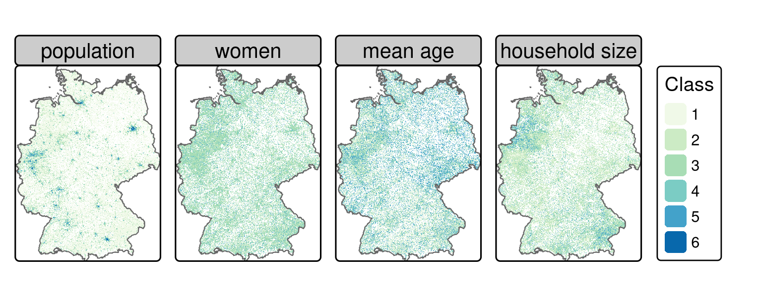
FIGURE 14.1: Gridded German census data of 2022 (women data from 2011). See Table 14.1 for reclassification thresholds.
The next stage is to reclassify the demographic variables (women, mean age, household size) into weights in accordance with the survey mentioned in Section 14.2, using the terra function classify(), which was introduced in Section 4.3.3.
Since Census 2022 provides actual continuous values rather than class codes, we can use the population counts directly without conversion. This gives us more precise data for delineating metropolitan areas (see Section 14.5).
For the remaining demographic variables, we reclassify continuous values into weights (0-3) based on our target audience criteria (see Table 14.1). Areas with 0-40% female population receive weight 3 because the target demographic is predominantly male. Similarly, areas with younger mean age and smaller household sizes receive higher weights.
# Reclassification matrices for continuous values (from, to, weight)
# Women: percentage of female inhabitants
rcl_women = matrix(c(
  0, 40, 3,    # 0-40% female -> weight 3
  40, 47, 2,   # 40-47% -> weight 2
  47, 53, 1,   # 47-53% -> weight 1
  53, 60, 0,   # 53-60% -> weight 0
  60, 100, 0   # >60% -> weight 0
), ncol = 3, byrow = TRUE)

# Mean age: continuous years
rcl_age = matrix(c(
  0, 40, 3,    # Mean age <40 -> weight 3
  40, 42, 2,   # 40-42 -> weight 2
  42, 44, 1,   # 42-44 -> weight 1
  44, 47, 0,   # 44-47 -> weight 0
  47, 120, 0   # >47 -> weight 0
), ncol = 3, byrow = TRUE)

# Household size: average persons per household
rcl_hh = matrix(c(
  0, 1.5, 3,     # 1-1.5 persons -> weight 3
  1.5, 2.0, 2,   # 1.5-2 -> weight 2
  2.0, 2.5, 1,   # 2-2.5 -> weight 1
  2.5, 3.0, 0,   # 2.5-3 -> weight 0
  3.0, 100, 0    # >3 -> weight 0
), ncol = 3, byrow = TRUE)

rcl = list(rcl_women, rcl_age, rcl_hh)
Note that we only reclassify women, mean age, and household size into weights — not population.
The for-loop applies each reclassification matrix to the corresponding raster layer.
We keep the population layer separate as actual counts for use in metropolitan area identification.
# Separate population (used as counts for metro detection) from variables to reclassify
pop_ras = input_ras$pop

# Reclassify women, mean_age, hh_size into weights
demo_vars = c("women", "mean_age", "hh_size")
reclass = input_ras[[demo_vars]]
for (i in seq_len(nlyr(reclass))) {
  reclass[[i]] = classify(x = reclass[[i]], rcl = rcl[[i]], right = NA)
}
names(reclass) = demo_vars
reclass # full output not shown
#> ...
#> names       : women, mean_age, hh_size
#> min values  :     0,        0,       0
#> max values  :     3,        3,       3
14.5 Define metropolitan areas
We deliberately define metropolitan areas as pixels of 20 km2 inhabited by more than 500,000 people.
Pixels at this coarse resolution can rapidly be created using aggregate(), as introduced in Section 5.3.3.
The command below uses the argument fact = 20 to reduce the resolution of the result 20-fold (recall the original raster resolution was 1 km2).
Since we have actual population counts from Census 2022 (rather than class-midpoint estimates), we can aggregate them directly.
pop_agg = aggregate(pop_ras, fact = 20, fun = sum, na.rm = TRUE)
summary(pop_agg)
#>       pop
#>  Min.   :     25
#>  1st Qu.:  22768
#>  Median :  45542
#>  Mean   :  82132
#>  3rd Qu.:  83074
#>  Max.   :1464047
#>  NAs    :412
The next stage is to keep only cells with more than half a million people.
pop_agg = pop_agg[pop_agg > 500000, drop = FALSE] Plotting this reveals several metropolitan regions (Figure 14.2).
Each region consists of one or more raster cells.
It would be nice if we could join all cells belonging to one region.
terra’s patches() command does exactly that.
Subsequently, as.polygons() converts the raster object into spatial polygons, and st_as_sf() converts it into an sf object.
metros = pop_agg |>
  patches(directions = 8) |>
  as.polygons() |>
  st_as_sf()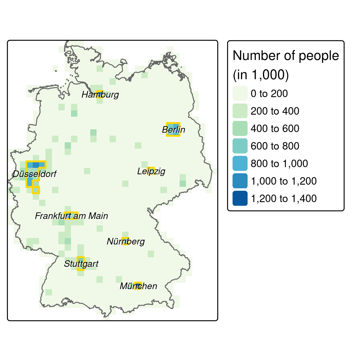
FIGURE 14.2: The aggregated population raster (resolution: 20 km) with the identified metropolitan areas (golden polygons) and the corresponding names.
The resulting metropolitan areas suitable for bike shops (Figure 14.2; see also code/14-location-figures.R for creating the figure) are still missing a name.
A reverse geocoding approach can settle this problem: given a coordinate, it finds the corresponding address.
Consequently, extracting the centroid coordinate of each metropolitan area can serve as an input for a reverse geocoding API.
This is exactly what the rev_geocode_OSM() function of the tmaptools package expects.
Setting additionally as.data.frame to TRUE will give back a data.frame with several columns referring to the location including the street name, house number and city.
However, here, we are only interested in the name of the city.
metro_names = sf::st_centroid(metros, of_largest_polygon = TRUE) |>
  tmaptools::rev_geocode_OSM(as.data.frame = TRUE) |>
  select(city, town, state)
# smaller cities are returned in column town. To have all names in one column,
# we move the town name to the city column in case it is NA
metro_names = dplyr::mutate(metro_names, city = ifelse(is.na(city), town, city))
To make sure that the reader uses the exact same results, we have put them into spDataLarge as the object metro_names.
| City | State |
|---|---|
| Hamburg | NA |
| Berlin | NA |
| Langenhagen | Niedersachsen |
| Wülfrath | Nordrhein-Westfalen |
| Leipzig | Sachsen |
| Dresden | Sachsen |
| Frankfurt am Main | Hessen |
| Nürnberg | Bayern |
| Stuttgart | Baden-Württemberg |
| München | Bayern |
Overall, we are satisfied with the City column serving as metropolitan names (Table 14.2) apart from two exceptions: Velbert belongs to the greater region of Düsseldorf, and Langenhagen belongs to Hannover.
Hence, we replace these names accordingly (Figure 14.2).
Umlauts like ü might lead to trouble further on, for example when determining the bounding box of a metropolitan area with opq() (see further below), which is why we avoid them.
metro_names = metro_names$city |>
  as.character() |>
  (\(x) ifelse(x == "Velbert", "Düsseldorf", x))() |>
  (\(x) ifelse(x == "Langenhagen", "Hannover", x))() |>
  gsub("ü", "ue", x = _)
14.6 Points of interest
The osmdata package provides easy-to-use access to OSM data (see also Section 8.5). Instead of downloading shops for the whole of Germany, we restrict the query to the defined metropolitan areas, reducing computational load and providing shop locations only in areas of interest. The subsequent code chunk does this using a number of functions including:
-
map()(the tidyverse equivalent oflapply()), which iterates through all metropolitan names which subsequently define the bounding box in the OSM query functionopq()(see Section 8.5) -
add_osm_feature()to specify OSM elements with a key value ofshop(see wiki.openstreetmap.org for a list of common key:value pairs) -
osmdata_sf(), which converts the OSM data into spatial objects (of classsf) -
while(), which tries two more times to download the data if the download failed the first time96
Before running this code, please consider it will download almost two GB of data.
To save time and resources, we have put the output named shops into spDataLarge.
To make it available in your environment, run data("shops", package = "spDataLarge").
shops = purrr::map(metro_names, function(x) {
  message("Downloading shops of: ", x, "\n")
  # give the server a bit time
  Sys.sleep(sample(seq(10, 15, 0.1), 1))
  query = osmdata::opq(x) |>
    osmdata::add_osm_feature(key = "shop")
  points = osmdata::osmdata_sf(query)
  # request the same data again if nothing has been downloaded
  iter = 2
  while (nrow(points$osm_points) == 0 && iter > 0) {
    points = osmdata_sf(query)
    iter = iter - 1
  }
  # return only the point features
  points$osm_points
})
It is highly unlikely that there are no shops in any of our defined metropolitan areas.
The following if condition simply checks if there is at least one shop for each region.
If not, we recommend to try to download the shops again for this/these specific region/s.
# checking if we have downloaded shops for each metropolitan area
ind = purrr::map_dbl(shops, nrow) == 0
if (any(ind)) {
  message("There are/is still (a) metropolitan area/s without any features:\n",
          paste(metro_names[ind], collapse = ", "), "\nPlease fix it!")
}
To make sure that each list element (an sf data frame) comes with the same columns97, we only keep the osm_id and the shop columns with the help of the map_dfr loop which additionally combines all shops into one large sf object.
# select only specific columns
shops = purrr::map_dfr(shops, select, osm_id, shop)
Note: shops is provided in the spDataLarge and can be accessed as follows:
data("shops", package = "spDataLarge")The only thing left to do is to convert the spatial point object into a raster (see Section 6.4).
The sf object, shops, is converted into a raster having the same parameters (dimensions, resolution, CRS) as the reclass object.
Importantly, the length() function is used here to count the number of shops in each cell.
The result of the subsequent code chunk is therefore an estimate of shop density (shops/km2).
st_transform() is used before rasterize() to ensure the CRS of both inputs match.
shops = sf::st_transform(shops, st_crs(reclass))
# create poi raster
poi = rasterize(x = shops, y = reclass, field = "osm_id", fun = "length")
As with the other raster layers (population, women, mean age, household size) the poi raster is reclassified into four classes (see Section 14.4).
Defining class intervals is an arbitrary undertaking to a certain degree.
One can use equal breaks, quantile breaks, fixed values or others.
Here, we choose the Fisher-Jenks natural breaks approach which minimizes within-class variance, the result of which provides an input for the reclassification matrix.
# construct reclassification matrix
int = classInt::classIntervals(values(poi), n = 4, style = "fisher")
int = round(int$brks)
rcl_poi = matrix(c(int[1], rep(int[-c(1, length(int))], each = 2),
                   int[length(int)] + 1), ncol = 2, byrow = TRUE)
rcl_poi = cbind(rcl_poi, 0:3)
# reclassify
poi = classify(poi, rcl = rcl_poi, right = NA)
names(poi) = "poi"
14.7 Identify suitable locations
The only step that remains before combining all the layers is to add poi to the reclass raster stack.
Note that we have already kept population separate from the demographic weights, as it was used only for delineating metropolitan areas.
The reasoning is: First, we have already identified areas where the population density is above average compared to the rest of Germany.
Second, though it is advantageous to have many potential customers within a specific catchment area, the sheer number alone might not actually represent the desired target group.
For instance, residential tower blocks are areas with a high population density but not necessarily with a high purchasing power for expensive cycle components.
# add poi raster to demographic weights
reclass = c(reclass, poi)
In common with other data science projects, data retrieval and ‘tidying’ have consumed much of the overall workload so far. With clean data, the final step — calculating a final score by summing all raster layers — can be accomplished in a single line of code.
# calculate the total score
result = sum(reclass)
For instance, a score of at least 9 might be a suitable threshold indicating raster cells where a bike shop could be placed (Figure 14.3; see also code/14-location-figures.R).
FIGURE 14.3: Suitable areas (i.e., raster cells with a score >= 9) in accordance with our hypothetical survey for bike stores in Berlin.
14.8 Discussion and next steps
The presented approach is a typical example of the normative usage of a GIS (Longley 2015). We combined survey data with expert-based knowledge and assumptions (definition of metropolitan areas, defining class intervals, definition of a final score threshold). This approach is less suitable for scientific research than applied analysis that provides an evidence-based indication of areas suitable for bike shops that should be compared with other sources of information. A number of changes to the approach could improve the analysis:
- We used equal weights when calculating the final scores but other factors, such as the household size, could be as important as the portion of women or the mean age
- We used all points of interest but only those related to bike shops, such as do-it-yourself, hardware, bicycle, fishing, hunting, motorcycles, outdoor and sports shops (see the range of shop values available on the OSM Wiki) may have yielded more refined results
- Data at a higher resolution may improve the output (see Exercises)
- We have used only a limited set of variables and data from other sources, such as the INSPIRE geoportal or data on cycle paths from OpenStreetMap, may enrich the analysis (see also Section 8.5)
- Interactions remained unconsidered, such as a possible relationship between the portion of men and single households
In short, the analysis could be extended in multiple directions. Nevertheless, it should have given you a first impression and understanding of how to obtain and deal with spatial data in R within a geomarketing context.
Finally, we have to point out that the presented analysis would be merely the first step of finding suitable locations. So far we have identified areas, 1 by 1 km in size, representing potentially suitable locations for a bike shop in accordance with our survey. Subsequent steps in the analysis could be taken:
- Find an optimal location based on number of inhabitants within a specific catchment area. For example, the shop should be reachable for as many people as possible within 15 minutes of traveling bike distance (catchment area routing). Thereby, we should account for the fact that the further away the people are from the shop, the more unlikely it becomes that they actually visit it (distance decay function)
- Also it would be a good idea to take into account competitors. That is, if there already is a bike shop in the vicinity of the chosen location, possible customers (or sales potential) should be distributed between the competitors (Huff 1963; Wieland 2017)
- We need to find suitable and affordable real estate, e.g., in terms of accessibility, availability of parking spots, desired frequency of passers-by, having big windows, etc.
14.9 Exercises
E1. This exercise requires the z22 package for accessing 100 m resolution data.
Install it with remotes::install_github("JsLth/z22").
Load the population data at 100 m cell resolution using z22::z22_data("population", res = "100m", year = 2022).
Aggregate it to a cell resolution of 1 km using terra::aggregate() with fun = sum, and compare the result with the 1 km resolution data from census_de.
Note that the 100 m data is much larger and may take some time to download.
E2. Suppose our bike shop predominantly sold electric bikes to older people. Change the age raster accordingly, repeat the remaining analyses and compare the changes with our original result.