8 Geographic data I/O
8.1 Introduction
This chapter is about reading and writing geographic data. Geographic data input is essential for geocomputation: real-world applications are impossible without data. Data output is also vital, enabling others to use valuable new or improved datasets resulting from your work. Taken together, these processes of input/output can be referred to as data I/O. Geographic data I/O is often done in haste at the beginning and end of projects and otherwise ignored. However, data import and export are fundamental to the success or otherwise of projects: small I/O mistakes made at the beginning of projects (e.g., using an out-of-date dataset) can lead to large problems down the line.
There are many geographic file formats, each with its own advantages and disadvantages, as described in Section 8.2. Reading and writing from and to these file formats is covered in Sections 8.3 and 8.4, respectively. In terms of where to find data, Section 8.5 describes geoportals and how to import data from them. Dedicated packages to ease geographic data import, from sources including OpenStreetMap, are described in Section 8.6. If you want to put your data ‘into production’ in web services (or if you want to be sure that your data adheres to established standards), geographic metadata is important, as described in Section 8.7. Another possibility to obtain spatial data is to use web services, outlined in Section 8.8. The final Section 8.9 demonstrates methods for saving visual outputs (maps), in preparation for Chapter 9 on visualization.
8.2 File formats
Geographic datasets are usually stored as files or in spatial databases. File formats can either store vector or raster data, while spatial databases such as PostGIS can store both (see also Section 10.7). Today the variety of file formats may seem bewildering, but there has been much consolidation and standardization since the beginnings of GIS software in the 1960s when the first widely distributed program (SYMAP) for spatial analysis was created at Harvard University (Coppock and Rhind 1991).
GDAL (which should be pronounced “goo-dal”, with the double “o” making a reference to object-orientation), Geospatial Data Abstraction Library, has resolved many issues associated with incompatibility between geographic file formats since its release in 2000. GDAL provides a unified and high-performance interface for reading and writing many raster and vector data formats.40 Many open and proprietary GIS programs, including GRASS GIS, ArcGIS and QGIS, use GDAL behind their GUIs for doing the legwork of ingesting and spitting out geographic data in appropriate formats.
GDAL provides access to more than 200 vector and raster data formats. Table 8.1 presents some basic information about selected and often used spatial file formats.
| Name | Extension | Information | Type | Model |
|---|---|---|---|---|
| ESRI Shapefile | .shp (the main file) | Popular format consisting of at least three files. No support for: files > 2 GB; mixed types; names > 10 chars; cols > 255. | Vector | Partially open |
| GeoJSON | .geojson | Extends the JSON exchange format by including a subset of the simple feature representation; mostly used for storing coordinates in longitude and latitude; it is extended by the TopoJSON format. | Vector | Open |
| KML | .kml | XML-based format for spatial visualization, developed for use with Google Earth. Zipped KML file forms the KMZ format. | Vector | Open |
| GPX | .gpx | XML schema created for exchange of GPS data. | Vector | Open |
| FlatGeobuf | .fgb | Single file format allowing for quick reading and writing of vector data. Has streaming capabilities. | Vector | Open |
| GeoTIFF | .tif/.tiff | Popular raster format. A TIFF file containing additional spatial metadata. | Raster | Open |
| Arc ASCII | .asc | Text format where the first six lines represent the raster header, followed by the raster cell values arranged in rows and columns. | Raster | Open |
| SQLite/SpatiaLite | .sqlite | Standalone relational database, SpatiaLite is the spatial extension of SQLite. | Vector and raster | Open |
| ESRI FileGDB | .gdb | Spatial and non-spatial objects created by ArcGIS. Allows multiple feature classes; topology. Limited support from GDAL. | Vector and raster | Proprietary |
| GeoPackage | .gpkg | Lightweight database container based on SQLite allowing an easy and platform-independent exchange of geodata. | Vector and (very limited) raster | Open |
An important development ensuring the standardization and open-sourcing of file formats was the founding of the Open Geospatial Consortium (OGC) in 1994. Beyond defining the simple features data model (see Section 2.2.1), the OGC also coordinates the development of open standards, for example as used in file formats such as GML, KML and GeoPackage. Open file formats of the kind endorsed by the OGC have several advantages over proprietary formats: the standards are published, ensure transparency and open up the possibility for users to further develop and adjust the file formats to their specific needs.
ESRI Shapefile is the most popular vector data exchange format; however, it is not an open format (though its specification is open). It was developed in the early 1990s and has a number of limitations. First of all, it is a multi-file format, which consists of at least three files. It only supports 255 columns, column names are restricted to ten characters and the file size limit is 2 GB. Furthermore, ESRI Shapefile does not support all possible geometry types, for example, it is unable to distinguish between a polygon and a multipolygon.41 Despite these limitations, a viable alternative had been missing for a long time. In recent years, GeoPackage emerged, and seems to be a more than suitable replacement candidate for ESRI Shapefile. Geopackage is a format for exchanging geospatial information and an OGC standard. The GeoPackage standard describes the rules on how to store geospatial information in a tiny SQLite container. Hence, GeoPackage is a lightweight spatial database container, which allows the storage of vector and raster data but also of non-spatial data and extensions. Aside from GeoPackage, there are other geospatial data exchange formats worth checking out (Table 8.1).
The GeoTIFF format seems to be the most prominent raster data format. It allows spatial information, such as CRS, to be embedded within a TIFF file. Similar to ESRI Shapefile, this format was first developed in the 1990s, but as an open format. Additionally, GeoTIFF is still being expanded and improved. One of the most significant recent additions to the GeoTIFF format is its variant called COG (Cloud Optimized GeoTIFF). Raster objects saved as COGs can be hosted on HTTP servers, so other people can read only parts of the file without downloading the whole file (see Sections 8.3.2 and 8.4.2).
There are many geographic file formats beyond those shown in Table 8.1 and new data formats capable of representing geographic are being developed. Recent examples are formats based on the GeoArrow and Zarr specifications. GDAL’s documentation provides a good resource for learning about other vector and raster drivers. Furthermore, some data formats can store other data models (types) beyond the vector and raster data models introduced in Section 2.2.1. It includes LAS and LAZ formats for storing lidar point clouds, and NetCDF and HDF for storing multidimensional arrays.
Spatial data is also often stored using tabular (non-spatial) text formats, including CSV files or Excel spreadsheets. For example, this can be convenient to share spatial samples with people who do not use GIS tools or exchange data with other software that does not accept spatial data formats. However, this approach has downsides: it is challenging for storing geometries that are more complex than POINTs and omits important spatial metadata such as the CRS.
8.3 Data input (I)
Executing commands such as sf::read_sf() (the main function we use for loading vector data) or terra::rast() (the main function used for loading raster data) silently sets off a chain of events that reads data from files.
Many R packages provide example datasets (e.g., the dataset spData::world that we used in earlier chapters) and functions to get geographic datasets from a range of data sources.
All of them load the data into R or, more precisely, assign objects to your workspace.
This means that when objects are imported into R they are stored in RAM42, can be listed with ls() (and should be viewable in ‘Environment’ panels in your development environement) and can be accessed from the .GlobalEnv of the R session.
8.3.1 Vector data
Spatial vector data comes in a wide variety of file formats.
Most popular representations such as .geojson and .gpkg files can be imported directly into R with the sf function read_sf() (or the equivalent st_read()), which uses GDAL’s vector drivers behind the scenes.
The st_drivers() function returns a data frame containing name and long_name in the first two columns, and features of each driver available to GDAL (and therefore sf), including ability to write data and store raster data in the subsequent columns, as illustrated for key file formats in Table 8.3.
| name | long_name | write | copy | is_raster | is_vector | vsi |
|---|---|---|---|---|---|---|
| ESRI Shapefile | ESRI Shapefile | TRUE | FALSE | FALSE | TRUE | TRUE |
| GPX | GPX | TRUE | FALSE | FALSE | TRUE | TRUE |
| KML | Keyhole Markup Language (KML) | TRUE | FALSE | FALSE | TRUE | TRUE |
| GeoJSON | GeoJSON | TRUE | FALSE | FALSE | TRUE | TRUE |
| GPKG | GeoPackage | TRUE | TRUE | TRUE | TRUE | TRUE |
| FlatGeobuf | FlatGeobuf | TRUE | FALSE | FALSE | TRUE | TRUE |
The following commands show the first three drivers reported the computer’s GDAL installation (results can vary depending on the GDAL version installed) and a summary of their features.
Note that the majority of drivers can write data, while only a dozen or so formats can efficiently represent raster data in addition to vector data (see ?st_drivers() for details):
sf_drivers = st_drivers()
head(sf_drivers, n = 3)
summary(sf_drivers[-c(1:2)])
The first argument of read_sf() is dsn, which should be a text string or an object containing a single text string.
The content of a text string could vary between different drivers.
In most cases, as with the ESRI Shapefile (.shp) or the GeoPackage format (.gpkg), the dsn would be a file name.
read_sf() guesses the driver based on the file extension, as illustrated for a .gpkg file below:
f = system.file("shapes/world.gpkg", package = "spData")
world = read_sf(f)
For some drivers, dsn could be provided as a folder name, access credentials for a database, or a GeoJSON string representation (see the examples of the read_sf() help page for more details).
Some vector driver formats can store multiple data layers.
By default, read_sf() automatically reads the first layer of the file specified in dsn; however, using the layer argument you can specify any other layer.
The read_sf() function also allows for reading just parts of the file into RAM with two possible mechanisms.
The first one is related to the query argument, which allows specifying what part of the data to read with the OGR SQL query text.
An example below extracts data for Tanzania only (Figure 8.1A).
It is done by specifying that we want to get all columns (SELECT *) from the "world" layer for which the name_long is equal to "Tanzania":
tanzania = read_sf(f, query = 'SELECT * FROM world WHERE name_long = "Tanzania"')If you do not know the names of the available columns, a good approach is to just read one row of the data with 'SELECT * FROM world WHERE FID = 1'.
FID represents a feature ID – most often, it is a row number; however, its values depend on the used file format.
For example, FID starts from 0 in ESRI Shapefile, from 1 in some other file formats, or can be even arbitrary.
The second mechanism uses the wkt_filter argument.
This argument expects a well-known text representing a study area for which we want to extract the data.
Let’s try it using a small example – we want to read polygons from our file that intersect with the buffer of 50,000 meters of Tanzania’s borders.
To do it, we need to prepare our “filter” by (a) creating the buffer (Section 5.2.3), (b) converting the sf buffer object into an sfc geometry object with st_geometry(), and (c) translating geometries into their well-known text representation with st_as_text():
tanzania_buf = st_buffer(tanzania, 50000)
tanzania_buf_geom = st_geometry(tanzania_buf)
tanzania_buf_wkt = st_as_text(tanzania_buf_geom)
Now, we can apply this “filter” using the wkt_filter argument.
tanzania_neigh = read_sf(f, wkt_filter = tanzania_buf_wkt)Our result, shown in Figure 8.1(B), contains Tanzania and every country within its 50-km buffer.
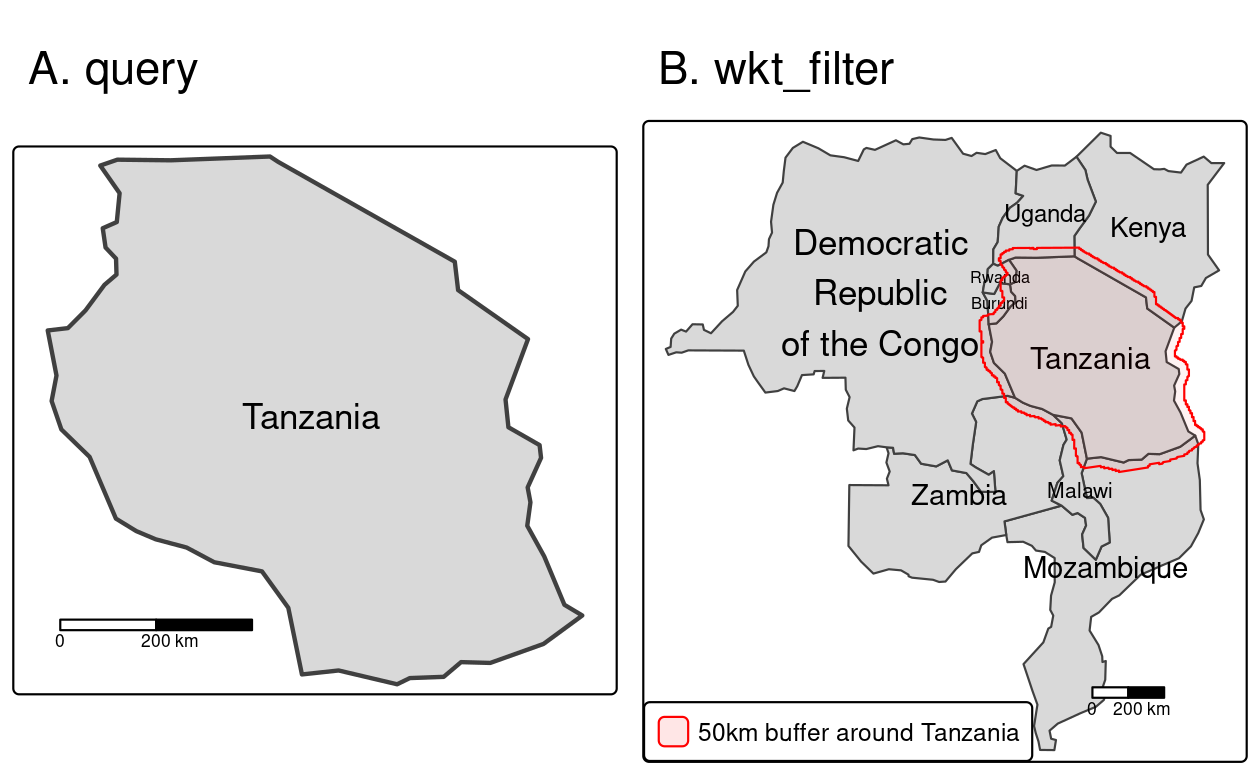
FIGURE 8.1: Reading a subset of the vector data using (A) a query and (B) a wkt filter.
Naturally, some options are specific to certain drivers.43
For example, think of coordinates stored in a spreadsheet format (.csv).
To read-in such files as spatial objects, we naturally have to specify the names of the columns (X and Y in our example below) representing the coordinates.
We can do this with the help of the options parameter.
To find out about possible options, please refer to the ‘Open Options’ section of the corresponding GDAL driver description.
For the comma-separated value (csv) format, visit https://gdal.org/drv_csv.html.
cycle_hire_txt = system.file("misc/cycle_hire_xy.csv", package = "spData")
cycle_hire_xy = read_sf(cycle_hire_txt,
  options = c("X_POSSIBLE_NAMES=X", "Y_POSSIBLE_NAMES=Y"))
Instead of columns describing ‘XY’ coordinates, a single column can also contain the geometry information.
Well-known text (WKT), well-known binary (WKB), and the GeoJSON formats are examples of this.
For instance, the world_wkt.csv file has a column named WKT representing polygons of the world’s countries.
We will again use the options parameter to indicate this.
world_txt = system.file("misc/world_wkt.csv", package = "spData")
world_wkt = read_sf(world_txt, options = "GEOM_POSSIBLE_NAMES=WKT")st_set_crs() function.
Please refer also to Section 7.3 for more information.
As a final example, we will show how read_sf() also reads KML files.
A KML file stores geographic information in XML format, which is a data format for the creation of web pages and the transfer of data in an application-independent way (Nolan and Lang 2014).
Here, we access a KML file from the web.
This file contains more than one layer.
st_layers() lists all available layers.
We choose the first layer Placemarks and say so with the help of the layer parameter in read_sf().
u = "https://developers.google.com/kml/documentation/KML_Samples.kml"
download.file(u, "KML_Samples.kml")
st_layers("KML_Samples.kml")
#> Driver: LIBKML
#> Available layers:
#>               layer_name geometry_type features fields crs_name
#> 1             Placemarks                      3     11   WGS 84
#> 2      Styles and Markup                      1     11   WGS 84
#> 3       Highlighted Icon                      1     11   WGS 84
....
kml = read_sf("KML_Samples.kml", layer = "Placemarks")
All the examples presented in this section so far have used the sf package for geographic data import. It is fast and flexible, but it may be worth looking at other packages such as duckdb, an R interface to the DuckDB database system which has a spatial extension.
8.3.2 Raster data
Similar to vector data, raster data comes in many file formats with some supporting multi-layer files.
terra’s rast() command reads in a single layer when a file with just one layer is provided.
raster_filepath = system.file("raster/srtm.tif", package = "spDataLarge")
single_layer = rast(raster_filepath)
It also works in case you want to read a multi-layer file.
multilayer_filepath = system.file("raster/landsat.tif", package = "spDataLarge")
multilayer_rast = rast(multilayer_filepath)
All of the previous examples read spatial information from files stored on your hard drive.
However, GDAL also allows reading data directly from online resources, such as HTTP/HTTPS/FTP web resources.
The only thing we need to do is to add a /vsicurl/ prefix before the path to the file.
This tells GDAL to use its virtual file system for network resources, which uses HTTP Range requests to fetch only the specific byte ranges needed for an operation rather than downloading the entire file.
Let’s try it by connecting to the global monthly snow probability at 500-m resolution for the period 2000-2012.
Snow probability for December is stored as a Cloud Optimized GeoTIFF (COG) file (see Section 8.2) at zenodo.org.
To read an online file, we just need to provide its URL together with the /vsicurl/ prefix.
myurl = paste0("/vsicurl/https://zenodo.org/record/5774954/files/",
               "clm_snow.prob_esacci.dec_p.90_500m_s0..0cm_2000..2012_v2.0.tif")
snow = rast(myurl)
snow
#> class       : SpatRaster
#> size        : 35849, 86400, 1  (nrow, ncol, nlyr)
#> resolution  : 0.004166667, 0.004166667  (x, y)
#> extent      : -180, 180, -62.00083, 87.37  (xmin, xmax, ymin, ymax)
#> coord. ref. : lon/lat WGS 84 (EPSG:4326)
#> source      : clm_snow.prob_esacci.dec_p.90_500m_s0..0cm_2000..2012_v2.0.tif
#> name        : clm_snow.prob_esacci.dec_p.90_500m_s0..0cm_2000..2012_v2.0
When combined with the /vsicurl/ prefix, COG files enable highly efficient remote data access.
Instead of reading the whole file into RAM, GDAL creates a connection that selectively fetches only the byte ranges needed for subsequent operations (e.g., crop() or extract()), making it possible to work with multi-gigabyte files over the internet almost as if they were local.
This allows us also to just read a tiny portion of the data without downloading the entire file.
For example, we can get the snow probability for December in Reykjavik (70%) by specifying its coordinates and applying the extract() function:
rey = data.frame(lon = -21.94, lat = 64.15)
snow_rey = extract(snow, rey)
snow_rey
#>   ID clm_snow.prob_esacci.dec_p.90_500m_s0..0cm_2000..2012_v2.0
#> 1  1                                                         70
This way, we just downloaded a single value instead of the whole, large GeoTIFF file.
The above example just shows one simple (but useful) case, but there is more to explore.
The /vsicurl/ prefix also works not only for raster but also for vector file formats.
It allows reading vectors directly from online storage with read_sf() just by adding the prefix before the vector file URL.
Importantly, /vsicurl/ is not the only prefix provided by GDAL – many more exist, such as /vsizip/ to read spatial files from ZIP archives without decompressing them beforehand or /vsis3/ for on-the-fly reading files available in AWS S3 buckets.
You can learn more about it at https://gdal.org/user/virtual_file_systems.html.
As with vector data, raster datasets can also be stored in and read from some spatial databases, notably PostGIS. See Section 10.7 for more details.
8.4 Data output (O)
Writing geographic data allows you to convert from one format to another and to save newly created objects.
Depending on the data type (vector or raster), object class (e.g., sf or SpatRaster), and type and amount of stored information (e.g., object size, range of values), it is important to know how to store spatial files in the most efficient way.
The next two sections will demonstrate how to do this.
8.4.1 Vector data
The counterpart of read_sf() is write_sf().
It allows you to write sf objects to a wide range of geographic vector file formats, including the most common such as .geojson, .shp and .gpkg.
Based on the file name, write_sf() decides automatically which driver to use.
The speed of the writing process depends also on the driver.
write_sf(obj = world, dsn = "world.gpkg")Note: if you try to write to the same data source again, the function will overwrite the file:
write_sf(obj = world, dsn = "world.gpkg")Instead of overwriting the file, we could add a new layer to the file by specifying the layer argument.
This is supported by several spatial formats, including GeoPackage.
write_sf(obj = world, dsn = "world_many_layers.gpkg", layer = "second_layer")Alternatively, you can use st_write() since it is equivalent to write_sf().
However, it has different defaults – it does not overwrite files (returns an error when you try to do it) and shows a short summary of the written file format and the object.
st_write(obj = world, dsn = "world2.gpkg")
#> Writing layer `world2' to data source `world2.gpkg' using driver `GPKG'
#> Writing 177 features with 10 fields and geometry type Multi Polygon.
The layer_options argument could be also used for many different purposes.
One of them is to write spatial data to a text file.
This can be done by specifying GEOMETRY inside of layer_options.
It could be either AS_XY for simple point datasets (it creates two new columns for coordinates) or AS_WKT for more complex spatial data (one new column is created which contains the well-known text representation of spatial objects).
8.4.2 Raster data
The writeRaster() function saves SpatRaster objects to files on disk.
The function expects input regarding output data type and file format, but also accepts GDAL options specific to a selected file format (see ?writeRaster for more details).
The terra package offers seven data types when saving a raster: INT1U, INT2S, INT2U, INT4S, INT4U, FLT4S, and FLT8S,44 which determine the bit representation of the raster object written to disk (Table 8.5).
Which data type to use depends on the range of the values of your raster object.
The more values a data type can represent, the larger the file will get on disk.
Unsigned integers (INT1U, INT2U, INT4U) are suitable for categorical data, while float numbers (FLT4S and FLT8S) usually represent continuous data.
writeRaster() uses FLT4S as the default.
While this works in most cases, the size of the output file will be unnecessarily large if you save binary or categorical data.
Therefore, we would recommend to use the data type that needs the least storage space but is still able to represent all values (check the range of values with the summary() function).
| Data Type | Minimum Value | Maximum Value |
|---|---|---|
| INT1U | 0 | 255 |
| INT2S | –32,767 | 32,767 |
| INT2U | 0 | 65,534 |
| INT4S | –2,147,483,647 | 2,147,483,647 |
| INT4U | 0 | 4,294,967,296 |
| FLT4S | –3.4e+38 | 3.4e+38 |
| FLT8S | –1.7e+308 | 1.7e+308 |
By default, the output file format is derived from the filename.
Naming a file *.tif will create a GeoTIFF file, as demonstrated below:
writeRaster(single_layer, filename = "my_raster.tif", datatype = "INT2U")Some raster file formats have additional options that can be set by providing GDAL parameters to the options argument of writeRaster().
GeoTIFF files are written in terra, by default, with the LZW compression gdal = c("COMPRESS=LZW").
To change or disable the compression, we need to modify this argument.
writeRaster(x = single_layer, filename = "my_raster.tif",
            gdal = c("COMPRESS=NONE"), overwrite = TRUE)
Additionally, we can save our raster object as COG (Cloud Optimized GeoTIFF, Section 8.2) with the filetype = "COG" options.
writeRaster(x = single_layer, filename = "my_raster.tif",
            filetype = "COG", overwrite = TRUE)
To learn more about the compression of GeoTIFF files, we recommend Paul Ramsey’s comprehensive blog post, GeoTiff Compression for Dummies which can be found online.
8.5 Geoportals
A vast and ever-increasing amount of geographic data is available on the internet, much of which is free to access and use (with appropriate credit given to its providers).45 In some ways there is now too much data, in the sense that there are often multiple places to access the same dataset. Some datasets are of poor quality. In this context, it is vital to know where to look, so the first section covers some of the most important sources. Various ‘geoportals’ (web services providing geospatial datasets such as Data.gov) are a good place to start, providing a wide range of data but often only for specific locations (as illustrated in the updated Wikipedia page on the topic).
Some global geoportals overcome this issue. The GEOSS portal and the Copernicus Data Space Ecosystem, for example, contain many raster datasets with global coverage. A wealth of vector datasets can be accessed from the SEDAC portal run by the National Aeronautics and Space Administration (NASA) and the European Union’s INSPIRE geoportal, with global and regional coverage.
Most geoportals provide a graphical interface allowing datasets to be queried based on characteristics such as spatial and temporal extent, the United States Geological Survey’s EarthExplorer being a prime example.
Exploring datasets interactively on a browser is an effective way of understanding available layers.
Downloading data is best done with code, however, from reproducibility and efficiency perspectives.
Downloads can be initiated from the command line using a variety of techniques, primarily via URLs and APIs (see the Copernicus APIs for example).46
Files hosted on static URLs can be downloaded with download.file(), as illustrated in the code chunk below which accesses PeRL: Permafrost Region Pond and Lake Database from pangaea.de:
download.file(url = "https://hs.pangaea.de/Maps/PeRL/PeRL_permafrost_landscapes.zip",
              destfile = "PeRL_permafrost_landscapes.zip",
              mode = "wb")
unzip("PeRL_permafrost_landscapes.zip")
canada_perma_land = read_sf("PeRL_permafrost_landscapes/canada_perma_land.shp")
8.6 Geographic data packages
Many R packages have been developed for accessing geographic data, some of which are presented in Table 8.6. These provide interfaces to one or more spatial libraries or geoportals and aim to make data access even quicker from the command line.
| Package | Description |
|---|---|
| climateR | Access over 100,000 gridded climate and landscape datasets from over 2,000 data providers by area of interest. |
| elevatr | Access point and raster elevation data from various sources. |
| FedData | Datasets maintained by the US federal government, including elevation and land cover. |
| geodata | Download and import imports administrative, elevation, WorldClim data. |
| osmdata | Download and import small OpenStreetMap datasets. |
| osmextract | Download and import large OpenStreetMap datasets. |
| rnaturalearth | Access Natural Earth vector and raster data. |
| rnoaa | Import National Oceanic and Atmospheric Administration (NOAA) climate data. |
It should be emphasized that Table 8.6 represents only a small number of available geographic data packages. For example, a large number of R packages exist to obtain various socio-demographic data, such as tidycensus and tigris (USA), cancensus (Canada), eurostat and giscoR (European Union), or idbr (international databases) – read Analyzing US Census Data (K. E. Walker 2022) to find some examples of how to analyze such data. Similarly, several R packages exist giving access to spatial data for various regions and countries, such as bcdata (Province of British Columbia), geobr (Brazil), RCzechia (Czech Republic), or rgugik (Poland).
Each data package has its own syntax for accessing data.
This diversity is demonstrated in the subsequent code chunks, which show how to get data using three packages from Table 8.6.47
Country borders are often useful and these can be accessed with the ne_countries() function from the rnaturalearth package (Massicotte and South 2023) as follows:
library(rnaturalearth)
usa_sf = ne_countries(country = "United States of America", returnclass = "sf")
Country borders can be also accessed with other packages, such as geodata, giscoR, or rgeoboundaries.
A second example downloads a series of rasters containing global monthly precipitation sums with spatial resolution of 10 minutes (~18.5 km at the equator) using the geodata package (Hijmans 2023a).
The result is a multi-layer object of class SpatRaster.
library(geodata)
worldclim_prec = worldclim_global("prec", res = 10, path = tempdir())
class(worldclim_prec)
A third example uses the osmdata package (Padgham et al. 2023) to find parks from the OpenStreetMap (OSM) database.
As illustrated in the code-chunk below, queries begin with the function opq() (short for OpenStreetMap query), the first argument of which is a bounding box, or text string representing a bounding box (the city of Leeds, in this case).
The result is passed to a function for selecting which OSM elements we’re interested in (parks in this case), represented by key-value pairs.
Next, they are passed to the function osmdata_sf() which does the work of downloading the data and converting it into a list of sf objects (see vignette('osmdata') for further details):
library(osmdata)
parks = opq(bbox = "leeds uk") |>
  add_osm_feature(key = "leisure", value = "park") |>
  osmdata_sf()
A limitation with the osmdata package is that it is rate-limited, meaning that it cannot download large OSM datasets (e.g., all the OSM data for a large city).
To overcome this limitation, the osmextract package was developed, which can be used to download and import binary .pbf files containing compressed versions of the OSM database for predefined regions.
OpenStreetMap is a vast global database of crowd-sourced data, is growing daily, and has a wider ecosystem of tools enabling easy access to the data, from the Overpass turbo web service for rapid development and testing of OSM queries to osm2pgsql for importing the data into a PostGIS database. Although the quality of datasets derived from OSM varies, the data source and wider OSM ecosystems have many advantages: they provide datasets that are available globally, free of charge, and constantly improving thanks to an army of volunteers. Using OSM encourages ‘citizen science’ and contributions back to the digital commons (you can start editing data representing a part of the world you know well at www.openstreetmap.org). Further examples of OSM data in action are provided in Chapters 10, 13 and 14.
Sometimes, packages come with built-in datasets.
These can be accessed in four ways: by attaching the package (if the package uses ‘lazy loading’ as spData does), with data(dataset, package = mypackage), by referring to the dataset with mypackage::dataset, or with system.file(filepath, package = mypackage) to access raw data files.
The following code chunk illustrates the latter two options using the world dataset (already loaded by attaching its parent package with library(spData)):48
world2 = spData::world
world3 = read_sf(system.file("shapes/world.gpkg", package = "spData"))
The last example, system.file("shapes/world.gpkg", package = "spData"), returns a path to the world.gpkg file, which is stored inside of the "shapes/" folder of the spData package.
Another way to obtain spatial information is to perform geocoding – transform a description of a location, usually an address, into its coordinates.
This is usually done by sending a query to an online service and getting the location as a result.
Many such services exist that differ in the used method of geocoding, usage limitations, costs, or application programming interface (API) key requirements.
R has several packages for geocoding; however, tidygeocoder seems to allow to connect to the largest number of geocoding services with a consistent interface.
The tidygeocoder main function is geocode, which takes a data frame with addresses and adds coordinates as "lat" and "long".
This function also allows to select a geocoding service with the method argument and has many additional parameters.
Let’s try this package by searching for coordinates of the John Snow blue plaque located on a building in the Soho district of London.
library(tidygeocoder)
geo_df = data.frame(address = "54 Frith St, London W1D 4SJ, UK")
geo_df = geocode(geo_df, address, method = "osm")
geo_df
The resulting data frame can be converted into an sf object with st_as_sf().
tidygeocoder also allows performing the opposite process called reverse geocoding used to get a set of information (name, address, etc.) based on a pair of coordinates. Geographic data can also be imported into R from various ‘bridges’ to geographic software, as described in Chapter 10.
8.7 Geographic metadata
Geographic metadata are a cornerstone of geographic information management, used to describe datasets, data structures and services. They help make datasets FAIR (Findable, Accessible, Interoperable, Reusable) and are defined by the ISO/OGC standards, in particular the ISO 19115 standard and underlying schemas. These standards are widely used within spatial data infrastructures, handled through metadata catalogs.
Geographic metadata can be managed with geometa, a package that allows writing, reading and validating geographic metadata according to the ISO/OGC standards. It already supports various international standards for geographic metadata information, such as the ISO 19110 (feature catalogue), legacy ISO 19115-1 and 19115-2 (geographic metadata for vector and gridded/imagery datasets), ISO 19115-3, ISO 19119 (geographic metadata for service), and ISO 19136 (Geographic Markup Language) providing methods to read, validate and write geographic metadata from R using the ISO/TS 19139 (XML) and ISO 19115-3 technical specifications. Geographic metadata can be created with geometa as follows, which creates and saves a metadata file:
library(geometa)
# create a metadata
md = ISOMetadata$new()
#... fill the metadata 'md' object
# validate metadata
md$validate()
# XML representation of the ISOMetadata
xml = md$encode()
# save metadata
md$save("my_metadata.xml")
# read a metadata from an XML file
md = readISO19139("my_metadata.xml")
The package comes with more examples and has been extended by packages such as geoflow to ease and automate the management of metadata.
In the field of standard geographic information management, the distinction between data and metadata is less clear. The Geography Markup Language (GML) standard and file format covers both data and metadata, for example. The geometa package allows exporting GML (ISO 19136) objects from geometry objects modeled with sf. Such functionality allows use of geographic metadata (enabling the inclusion of metadata on detailed geographic and temporal extents, rather than simple bounding boxes, for example) and the provision of services that extend the GML standard (e.g., Open Geospatial Consortium Web Coverage Service, OGC-WCS).
8.8 Geographic web services
In an effort to standardize web APIs for accessing spatial data, the Open Geospatial Consortium (OGC) has created a number of standard specifications for web services (collectively known as OWS, which is short for OGC Web Services). These services complement and use core standards developed to model geographic information, such as the ISO/OGC Spatial Schema (ISO 19107:2019), or the Simple Features (ISO 19125-1:2004), and to format data, such as with the Geographic Markup Language (GML). These specifications cover common access services for data and metadata. Vector data can be accessed with the Web Feature Service (WFS), whereas grid/imagery can be accessed with the Web Coverage Service (WCS). Map image representations, such as tiles, can be accessed with the Web Map Service (WMS) or the Web Map Tile Service (WMTS). Metadata is also covered by means of the Catalogue Service for the Web (CSW). Finally, standard processing is handled through the Web Processing Service (WPS) or the the Web Coverage Processing Service (WCPS).
Various open-source projects have adopted these protocols, such as GeoServer and MapServer for data-handling, or GeoNetwork and PyCSW for metadata-handling, leading to standardization of queries. Integrated tools for Spatial Data Infrastructures (SDI), such as GeoNode, GeOrchestra or Examind have also adopted these standard webservices, either directly or by using previously mentioned open-source tools.
Like other web APIs, OWS APIs use a ‘base URL’, an ‘endpoint’ and ‘URL query arguments’ following a ? to request data (see the best-practices-api-packages vignette in the httr package).
There are many requests that can be made to a OWS service. Below examples illustrate how some requests can be made directly with httr or more straightforward with the ows4R package (OGC Web-Services for R).
Let’s start with examples using the httr package, which can be useful for understanding how web services work.
One of the most fundamental requests is getCapabilities, demonstrated with httr functions GET() and modify_url() below.
The following code chunk demonstrates how API queries can be constructed and dispatched, in this case to discover the capabilities of a service run by the Fisheries and Aquaculture Division of the Food and Agriculture Organization of the United Nations (UN-FAO).
library(httr)
base_url = "https://www.fao.org"
endpoint = "/fishery/geoserver/wfs"
q = list(request = "GetCapabilities")
res = GET(url = modify_url(base_url, path = endpoint), query = q)
res$url
#> [1] "https://www.fao.org/fishery/geoserver/wfs?request=GetCapabilities"
The above code chunk demonstrates how API requests can be constructed programmatically with the GET() function, which takes a base URL and a list of query parameters that can easily be extended.
The result of the request is saved in res, an object of class response defined in the httr package, which is a list containing information of the request, including the URL.
As can be seen by executing browseURL(res$url), the results can also be read directly in a browser.
One way of extracting the contents of the request is as follows:
txt = content(res, "text")
xml = xml2::read_xml(txt)
xml
#> {xml_document} ...
#> [1] <ows:ServiceIdentification>\n  <ows:Title>GeoServer WFS...
#> [2] <ows:ServiceProvider>\n  <ows:ProviderName>UN-FAO Fishe...
#> ...
Data can be downloaded from WFS services with the GetFeature request and a specific typeName (as illustrated in the code chunk below).
Available names differ depending on the accessed web feature service.
One can extract them programmatically using web technologies (Nolan and Lang 2014) or scrolling manually through the contents of the GetCapabilities output in a browser.
library(sf)
sf::sf_use_s2(FALSE)
qf = list(request = "GetFeature", typeName = "fifao:FAO_MAJOR")
file = tempfile(fileext = ".gml")
GET(url = base_url, path = endpoint, query = qf, write_disk(file))
fao_areas = read_sf(file)
In order to keep geometry validity along the data access chain, and since standards and underlying open-source server solutions (such as GeoServer) have been built on the Simple Features access, it is important to deactivate the new default behavior introduced in sf, and to not use the S2 geometry model at data access time.
This is done with above code sf::sf_use_s2(FALSE).
Also note the use of write_disk() to ensure that the results are written to disk rather than loaded into memory, allowing them to be imported with sf.
For many everyday tasks, however, a higher-level interface may be more appropriate, and a number of R packages, and tutorials, have been developed precisely for this purpose. The package ows4R has been developed for working with OWS services. It provides a stable interface to common access services, such as the WFS, WCS for data, CSW for metadata, and WPS for processing. The OGC services coverage is described in the README of the package, hosted at github.com/eblondel/ows4R, with new standard protocols under investigation/development.
Based on the above example, the code below shows how to perform getCapabilities and getFeatures operations with this package.
The ows4R package relies on the principle of clients.
To interact with an OWS service (such as WFS), a client is created as follows:
library(ows4R)
WFS = WFSClient$new(
  url = "https://www.fao.org/fishery/geoserver/wfs",
  serviceVersion = "1.0.0",
  logger = "INFO"
)
The operations are then accessible from this client object, e.g., getCapabilities or getFeatures.
As explained before, when accessing data with OGC services, handling sf features should be done by deactivating the new default behavior introduced in sf, with sf::sf_use_s2(FALSE).
This is done by default with ows4R.
Additional examples are available through vignettes, such as how to access raster data with the WCS, or how to access metadata with the CSW.
8.9 Visual outputs
R supports many different static and interactive graphics formats. Chapter 9 covers map-making in detail, but it is worth mentioning ways to output visualizations here. The most general method to save a static plot is to open a graphic device, create a plot, and close it, for example:
Other available graphic devices include pdf(), bmp(), jpeg(), and tiff().
You can specify several properties of the output plot, including width, height and resolution.
Additionally, several graphic packages provide their own functions to save a graphical output.
For example, the tmap package has the tmap_save() function.
You can save a tmap object to different graphic formats or an HTML file by specifying the object name and a file path to a new file.
library(tmap)
tmap_obj = tm_shape(world) + tm_polygons(col = "lifeExp")
tmap_save(tmap_obj, filename = "lifeExp_tmap.png")
On the other hand, you can save interactive maps created in the mapview package as an HTML file or image using the mapshot2() function:
8.10 Exercises
E1. List and describe three types of vector, raster, and geodatabase formats.
E2. Name at least two differences between the sf functions read_sf() and st_read().
E3. Read the cycle_hire_xy.csv file from the spData package as a spatial object (Hint: it is located in the misc folder).
What is a geometry type of the loaded object?
E4. Download the borders of Germany using rnaturalearth, and create a new object called germany_borders.
Write this new object to a file of the GeoPackage format.
E5. Download the global monthly minimum temperature with a spatial resolution of 5 minutes using the geodata package.
Extract the June values, and save them to a file named tmin_june.tif file (hint: use terra::subset()).
E6. Create a static map of Germany’s borders, and save it to a PNG file.
E7. Create an interactive map using data from the cycle_hire_xy.csv file.
Export this map to a file called cycle_hire.html.