5 Geometry operations

library(sf)
library(terra)
library(dplyr)
library(spData)
library(spDataLarge)

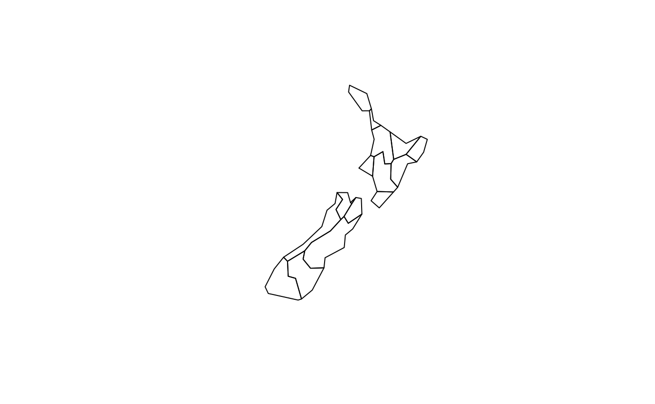
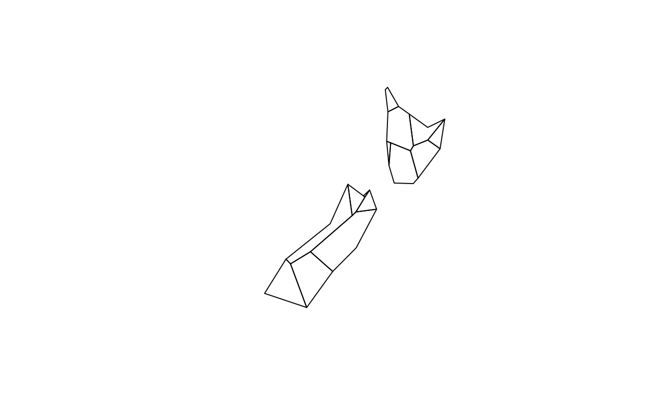
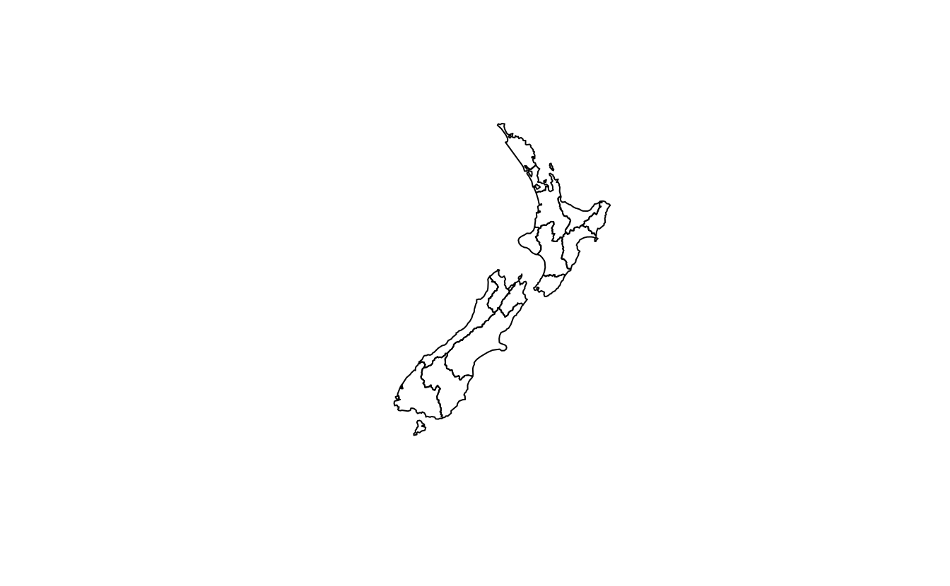
E1. Generate and plot simplified versions of the nz dataset. Experiment with different values of keep (ranging from 0.5 to 0.00005) for ms_simplify() and dTolerance (from 100 to 100,000) st_simplify().

At what value does the form of the result start to break down for each method, making New Zealand unrecognizable?
Advanced: What is different about the geometry type of the results from st_simplify() compared with the geometry type of ms_simplify()? What problems does this create and how can this be resolved?

plot(rmapshaper::ms_simplify(st_geometry(nz), keep = 0.5))
plot(rmapshaper::ms_simplify(st_geometry(nz), keep = 0.05))
# Starts to breakdown here at 0.5% of the points:
plot(rmapshaper::ms_simplify(st_geometry(nz), keep = 0.005))
# At this point no further simplification changes the result
plot(rmapshaper::ms_simplify(st_geometry(nz), keep = 0.0005))
plot(rmapshaper::ms_simplify(st_geometry(nz), keep = 0.00005))
plot(st_simplify(st_geometry(nz), dTolerance = 100))
plot(st_simplify(st_geometry(nz), dTolerance = 1000))
# Starts to breakdown at 10 km:
plot(st_simplify(st_geometry(nz), dTolerance = 10000))
plot(st_simplify(st_geometry(nz), dTolerance = 100000))
plot(st_simplify(st_geometry(nz), dTolerance = 100000, preserveTopology = TRUE))

# Problem: st_simplify returns POLYGON and MULTIPOLYGON results, affecting plotting
# Cast into a single geometry type to resolve this
nz_simple_poly = st_simplify(st_geometry(nz), dTolerance = 10000) |> 
  st_sfc() |> 
  st_cast("POLYGON")
#> Warning in st_cast.MULTIPOLYGON(X[[i]], ...): polygon from first part only
#> Warning in st_cast.MULTIPOLYGON(X[[i]], ...): polygon from first part only
nz_simple_multipoly = st_simplify(st_geometry(nz), dTolerance = 10000) |> 
  st_sfc() |> 
  st_cast("MULTIPOLYGON")
plot(nz_simple_poly)
length(nz_simple_poly)
#> [1] 16
nrow(nz)
#> [1] 16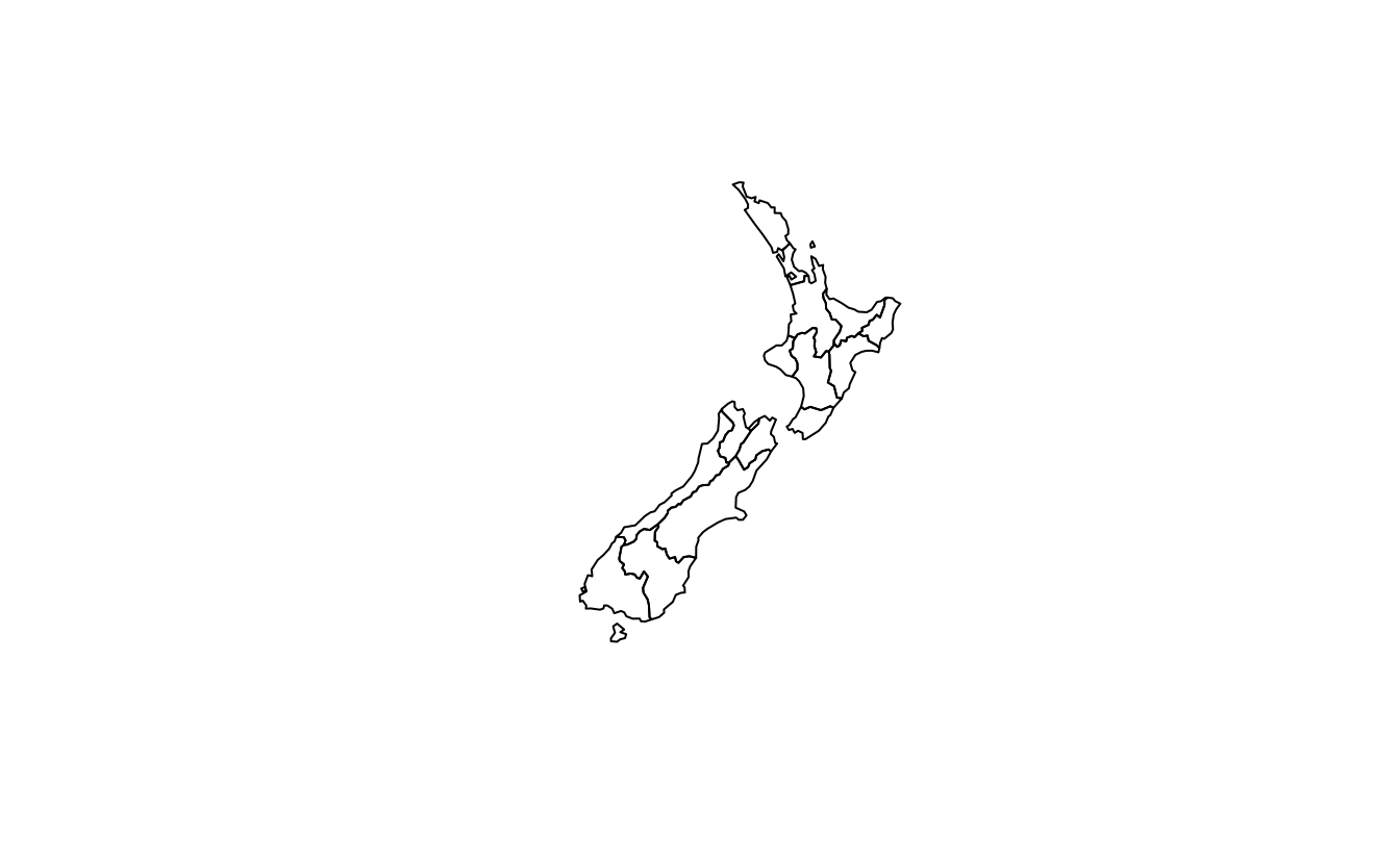

E2. In the first exercise in Chapter Spatial Data Operations it was established that Canterbury region had 70 of the 101 highest points in New Zealand. Using st_buffer(), how many points in nz_height are within 100 km of Canterbury?

canterbury = nz[nz$Name == "Canterbury", ]
cant_buff = st_buffer(canterbury, 100000)
nz_height_near_cant = nz_height[cant_buff, ]
nrow(nz_height_near_cant) # 75 - 5 more
#> [1] 95

E3. Find the geographic centroid of New Zealand. How far is it from the geographic centroid of Canterbury?

cant_cent = st_centroid(canterbury)
#> Warning: st_centroid assumes attributes are constant over geometries
nz_centre = st_centroid(st_union(nz))
st_distance(cant_cent, nz_centre) # 234 km
#> Units: [m]
#>        [,1]
#> [1,] 234193

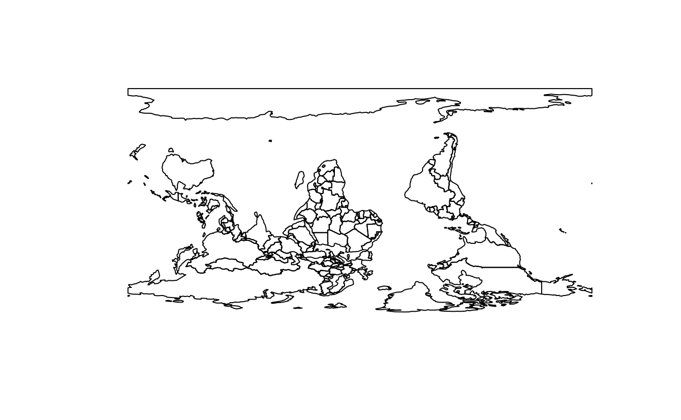
E4. Most world maps have a north-up orientation. A world map with a south-up orientation could be created by a reflection (one of the affine transformations not mentioned in this chapter) of the world object’s geometry. Write code to do so. Hint: you can to use the rotation() function from this chapter for this transformation. Bonus: create an upside-down map of your country.

rotation = function(a){
  r = a * pi / 180 #degrees to radians
  matrix(c(cos(r), sin(r), -sin(r), cos(r)), nrow = 2, ncol = 2)
} 

world_sfc = st_geometry(world)
world_sfc_mirror = world_sfc * rotation(180)
plot(world_sfc)
plot(world_sfc_mirror)

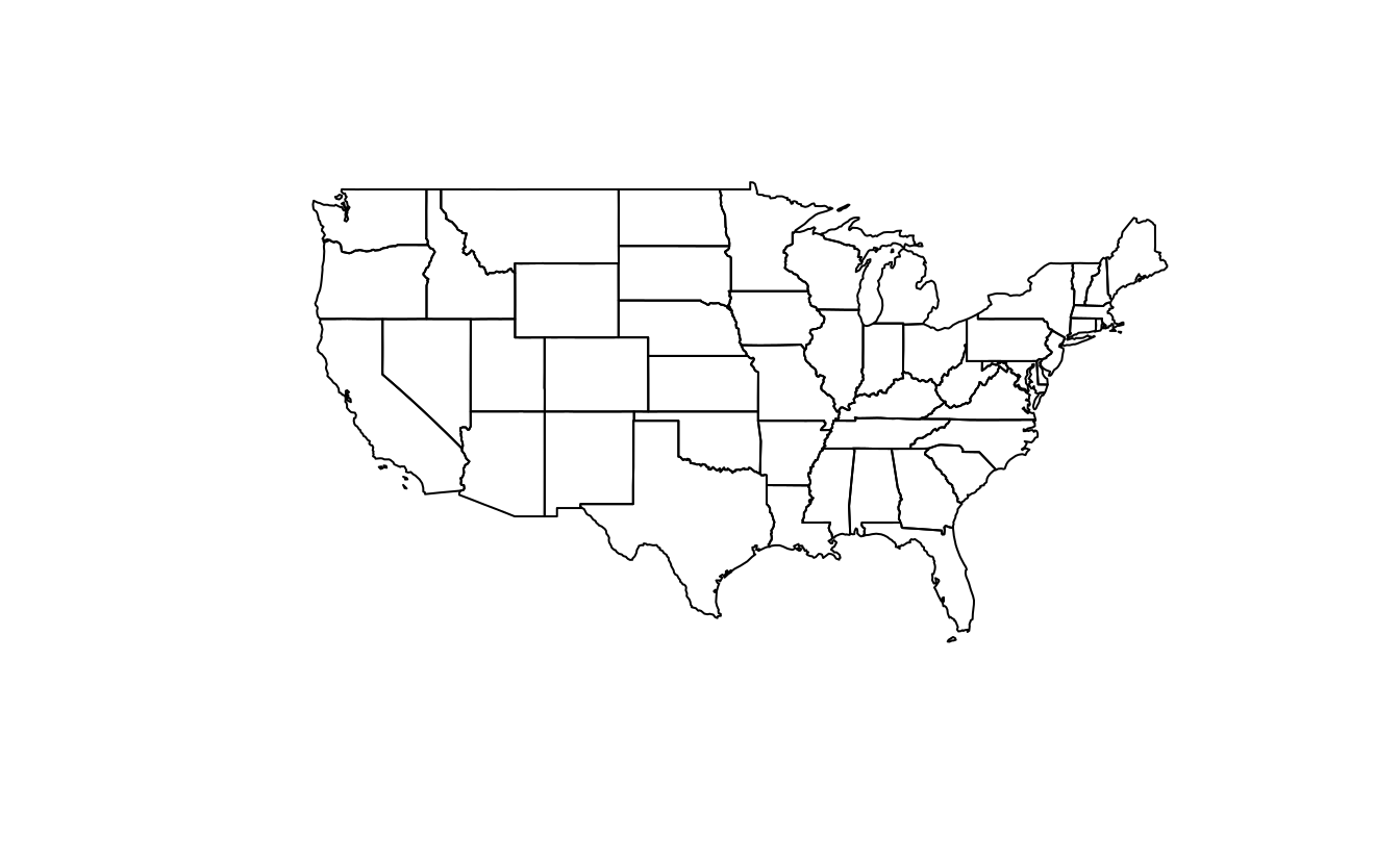
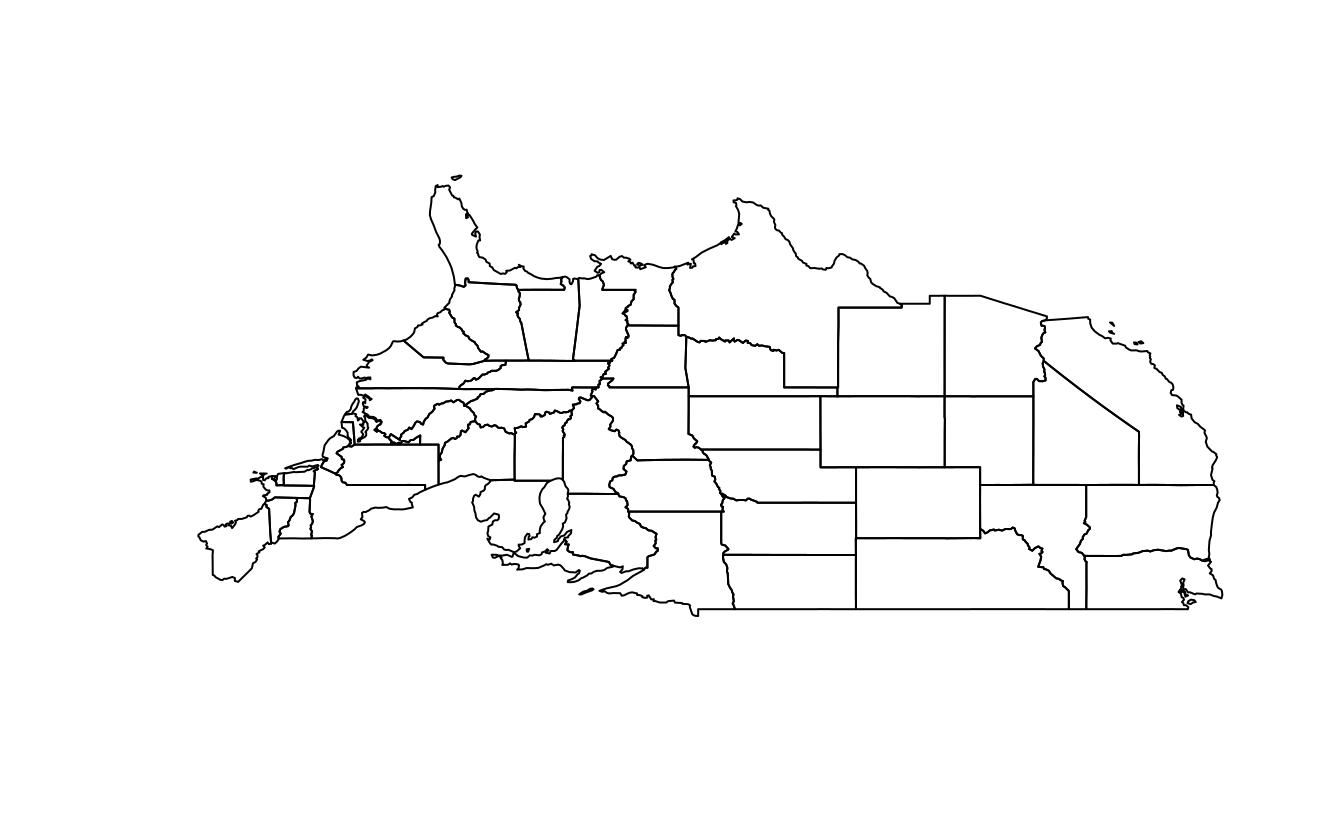
us_states_sfc = st_geometry(us_states)
us_states_sfc_mirror = us_states_sfc * rotation(180)
plot(us_states_sfc)
plot(us_states_sfc_mirror)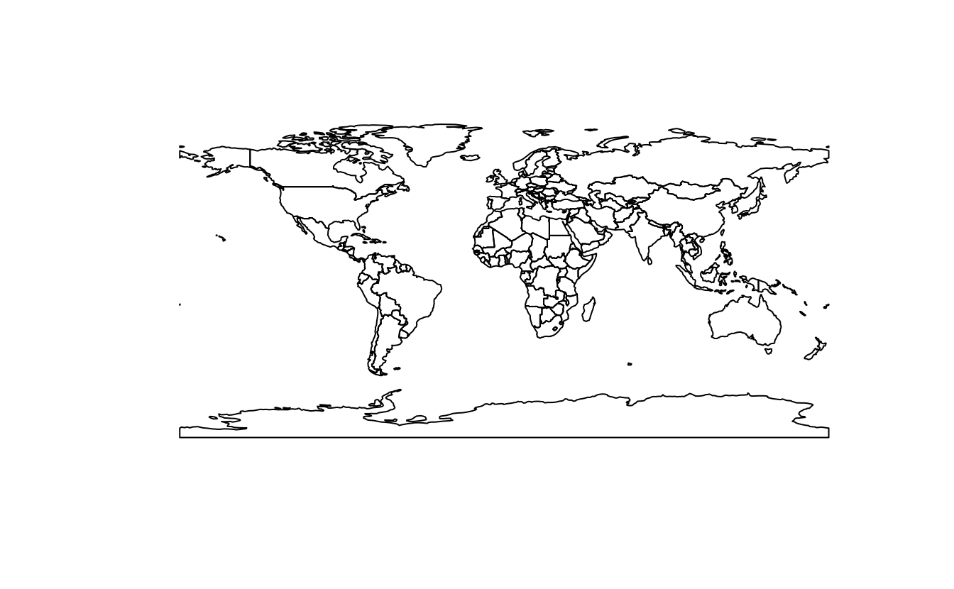

E5. Run the code in Section 5.2.6. With reference to the objects created in that section, subset the point in p that is contained within x and y.

Using base subsetting operators.
Using an intermediary object created with st_intersection().

p_in_y = p[y]
p_in_xy = p_in_y[x]
x_and_y = st_intersection(x, y)
p[x_and_y]
#> Geometry set for 1 feature 
#> Geometry type: POINT
#> Dimension:     XY
#> Bounding box:  xmin: 0.305 ymin: 1.43 xmax: 0.305 ymax: 1.43
#> CRS:           NA
#> POINT (0.305 1.43)

E6. Calculate the length of the boundary lines of US states in meters. Which state has the longest border and which has the shortest? Hint: The st_length function computes the length of a LINESTRING or MULTILINESTRING geometry.

us_states9311 = st_transform(us_states, "EPSG:9311")
us_states_bor = st_cast(us_states9311, "MULTILINESTRING")
us_states_bor$borders = st_length(us_states_bor)
arrange(us_states_bor, borders)
#> Simple feature collection with 49 features and 7 fields
#> Geometry type: MULTILINESTRING
#> Dimension:     XY
#> Bounding box:  xmin: -2040000 ymin: -2110000 xmax: 2520000 ymax: 731000
#> Projected CRS: NAD27 / US National Atlas Equal Area
#> First 10 features:
#>    GEOID                 NAME   REGION         AREA total_pop_10 total_pop_15
#> 1     11 District of Columbia    South   178 [km^2]       584400       647484
#> 2     44         Rhode Island Norteast  2743 [km^2]      1056389      1053661
#> 3     10             Delaware    South  5182 [km^2]       881278       926454
#> 4     09          Connecticut Norteast 12977 [km^2]      3545837      3593222
#> 5     34           New Jersey Norteast 20274 [km^2]      8721577      8904413
#> 6     50              Vermont Norteast 24866 [km^2]       624258       626604
#> 7     33        New Hampshire Norteast 24026 [km^2]      1313939      1324201
#> 8     25        Massachusetts Norteast 20911 [km^2]      6477096      6705586
#> 9     45       South Carolina    South 80904 [km^2]      4511428      4777576
#> 10    18              Indiana  Midwest 93648 [km^2]      6417398      6568645
#>        borders                       geometry
#> 1    60330 [m] MULTILINESTRING ((1955479 -...
#> 2   304697 [m] MULTILINESTRING ((2338362 4...
#> 3   407939 [m] MULTILINESTRING ((2041302 -...
#> 4   514571 [m] MULTILINESTRING ((2148010 2...
#> 5   747090 [m] MULTILINESTRING ((2062773 -...
#> 6   778660 [m] MULTILINESTRING ((2054045 3...
#> 7   782892 [m] MULTILINESTRING ((2188613 3...
#> 8  1018656 [m] MULTILINESTRING ((2422968 3...
#> 9  1275538 [m] MULTILINESTRING ((1534988 -...
#> 10 1436255 [m] MULTILINESTRING ((1033797 -...
arrange(us_states_bor, -borders)
#> Simple feature collection with 49 features and 7 fields
#> Geometry type: MULTILINESTRING
#> Dimension:     XY
#> Bounding box:  xmin: -2040000 ymin: -2110000 xmax: 2520000 ymax: 731000
#> Projected CRS: NAD27 / US National Atlas Equal Area
#> First 10 features:
#>    GEOID       NAME  REGION          AREA total_pop_10 total_pop_15     borders
#> 1     48      Texas   South 687714 [km^2]     24311891     26538614 4959186 [m]
#> 2     06 California    West 409747 [km^2]     36637290     38421464 3810350 [m]
#> 3     26   Michigan Midwest 151119 [km^2]      9952687      9900571 3579183 [m]
#> 4     12    Florida   South 151052 [km^2]     18511620     19645772 2949048 [m]
#> 5     30    Montana    West 380829 [km^2]       973739      1014699 2826586 [m]
#> 6     16      Idaho    West 216513 [km^2]      1526797      1616547 2570606 [m]
#> 7     27  Minnesota Midwest 218566 [km^2]      5241914      5419171 2567386 [m]
#> 8     51   Virginia   South 105405 [km^2]      7841754      8256630 2407299 [m]
#> 9     35 New Mexico    West 314886 [km^2]      2013122      2084117 2378172 [m]
#> 10    53 Washington    West 175436 [km^2]      6561297      6985464 2344358 [m]
#>                          geometry
#> 1  MULTILINESTRING ((-269579 -...
#> 2  MULTILINESTRING ((-1720565 ...
#> 3  MULTILINESTRING ((1113866 1...
#> 4  MULTILINESTRING ((1855611 -...
#> 5  MULTILINESTRING ((-1165102 ...
#> 6  MULTILINESTRING ((-1298509 ...
#> 7  MULTILINESTRING ((202873 44...
#> 8  MULTILINESTRING ((2104821 -...
#> 9  MULTILINESTRING ((-805019 -...
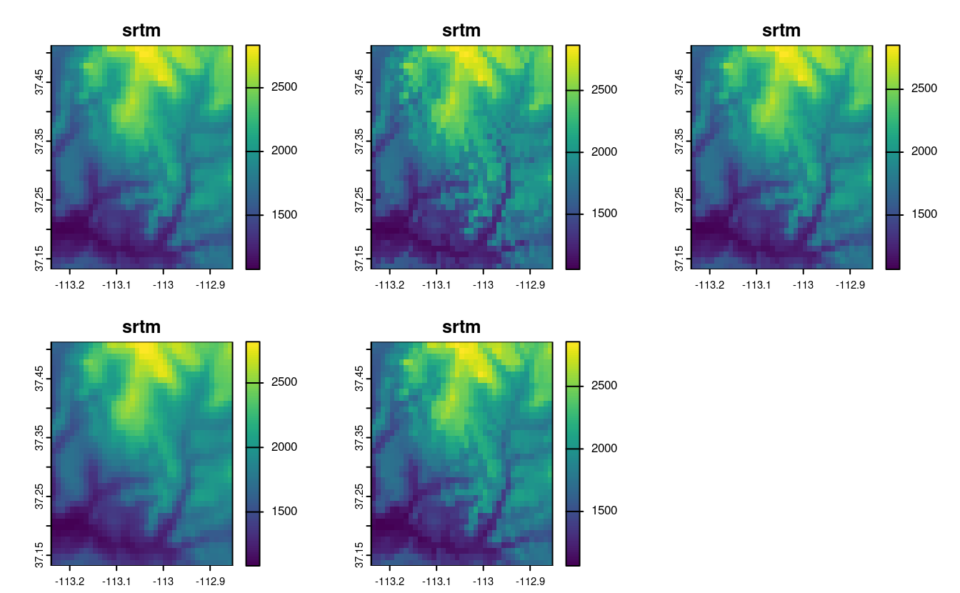
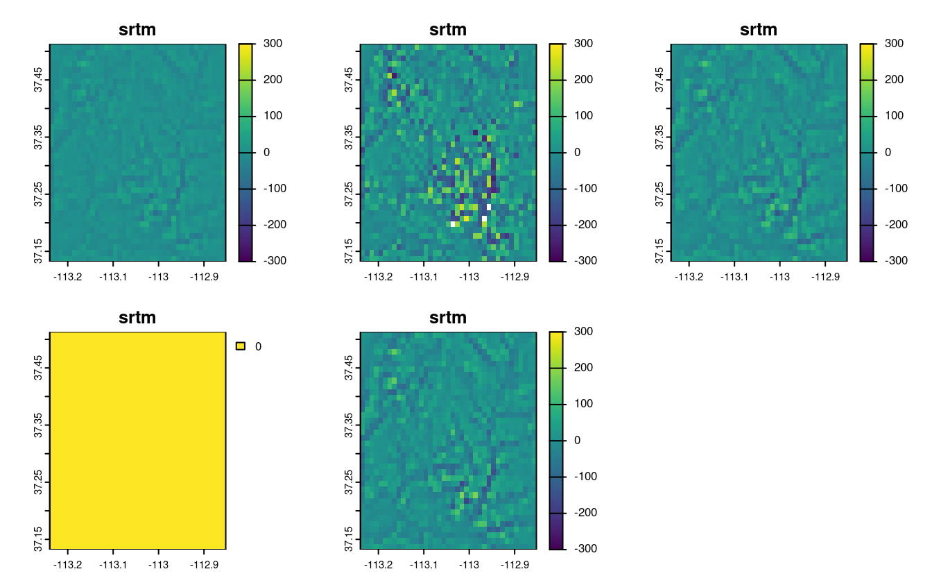
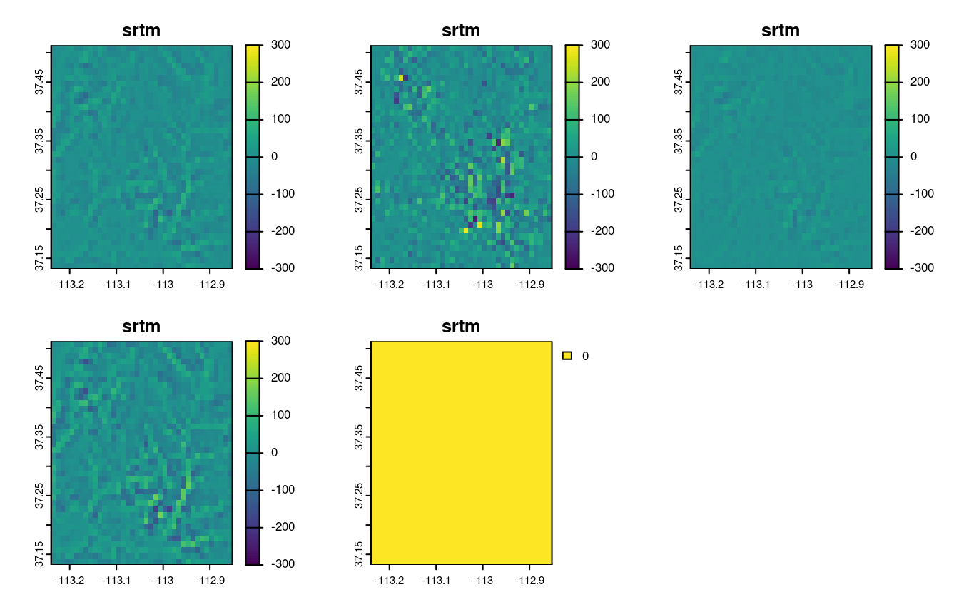
#> 10 MULTILINESTRING ((-1663690 ...

E7. Read the srtm.tif file into R (srtm = rast(system.file("raster/srtm.tif", package = "spDataLarge"))). This raster has a resolution of 0.00083 * 0.00083 degrees. Change its resolution to 0.01 * 0.01 degrees using all of the methods available in the terra package. Visualize the results. Can you notice any differences between the results of these resampling methods?

srtm = rast(system.file("raster/srtm.tif", package = "spDataLarge"))
rast_template = rast(ext(srtm), res = 0.01)
srtm_resampl1 = resample(srtm, y = rast_template, method = "bilinear")
srtm_resampl2 = resample(srtm, y = rast_template, method = "near")
srtm_resampl3 = resample(srtm, y = rast_template, method = "cubic")
srtm_resampl4 = resample(srtm, y = rast_template, method = "cubicspline")
srtm_resampl5 = resample(srtm, y = rast_template, method = "lanczos")

srtm_resampl_all = c(srtm_resampl1, srtm_resampl2, srtm_resampl3,
                     srtm_resampl4, srtm_resampl5)
plot(srtm_resampl_all)

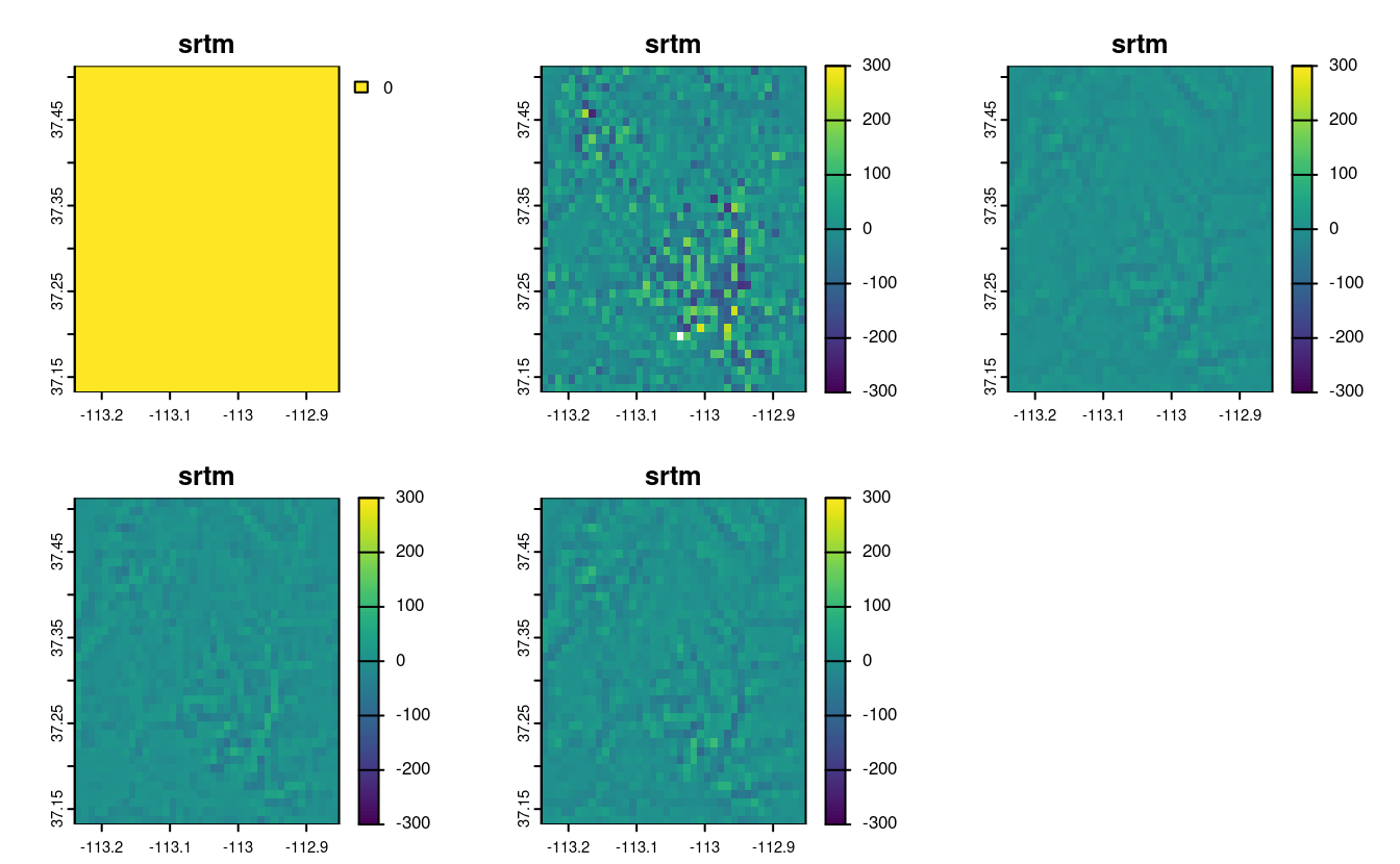
# differences
plot(srtm_resampl_all - srtm_resampl1, range = c(-300, 300))
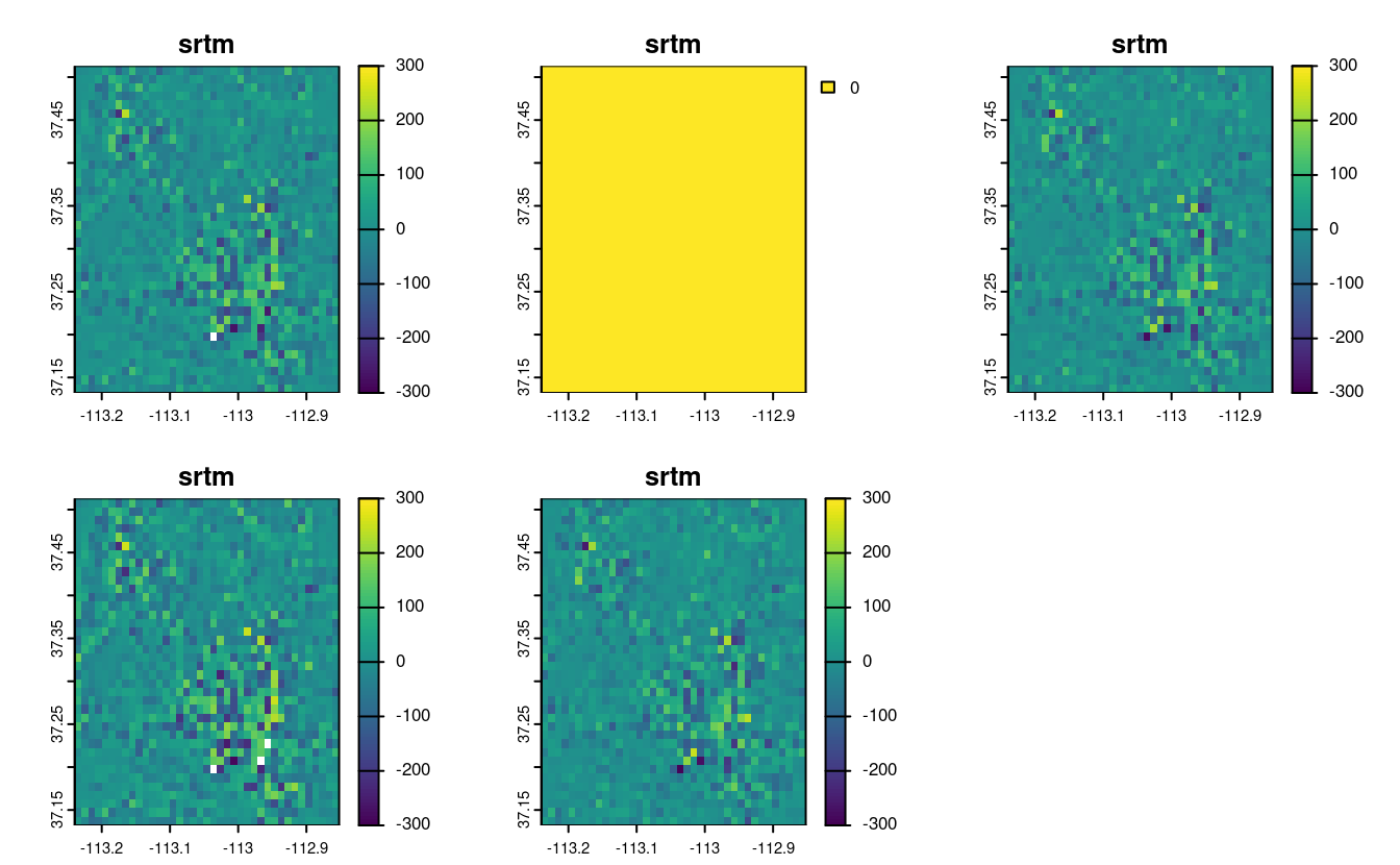
plot(srtm_resampl_all - srtm_resampl2, range = c(-300, 300))
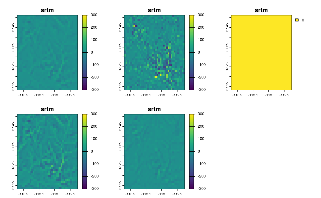
plot(srtm_resampl_all - srtm_resampl3, range = c(-300, 300))
plot(srtm_resampl_all - srtm_resampl4, range = c(-300, 300))
plot(srtm_resampl_all - srtm_resampl5, range = c(-300, 300))

4 Spatial data operations

6 Raster-vector interactions

Geocomputation with R: Solutions

5 Geometry operations

Solutions to the Second Edition's exercises